Match Outcome Prediction Using Logistic Regression in PyTorch
Introduction
This analysis is the final project of the course Introduction to Neural Networks and PyTorch by IBM.
League of Legends, a popular multiplayer online battle arena (MOBA) game, generates extensive data from matches. This project builds a logistic regression model that aimed at predicting the outcomes of League of Legends matches.
Data: league_of_legends_data_large.csv
Step 1: Data Loading and Preprocessing
Task 1: Load the League of Legends dataset and preprocess it for training.
Loading and preprocessing the dataset involves reading the data, splitting it into training and testing sets, and standardizing the features. You will utilize pandas for data manipulation, train_test_split from sklearn for data splitting, and StandardScaler for feature scaling.
- Load the dataset:
- Use
pd.read_csv()to load the dataset into a pandas DataFrame.
- Use
- Split data into features and target: Separate win (target) and the remaining columns (features).
- X = data.drop(‘win’, axis=1)
- y = data[‘win’] 3 .Split the Data into Training and Testing Sets:
- Use
train_test_split()fromsklearn.model_selectionto divide the data. Settest_size=0.2 to allocate 20% for testing and 80% for training, and userandom_state=42 to ensure reproducibility of the split.
- Standardize the features:
- Use
StandardScaler()from sklearn.preprocessing to scale the features.
- Use
- Convert to PyTorch tensors:
- Use
torch.tensor()to convert the data to PyTorch tensors.
- Use
Task 1: Implementation
Write code to load the dataset, split it into training and testing sets, standardize the features, and convert the data into PyTorch tensors for use in training a PyTorch model.
# Installing required libraries
!pip install pandas
!pip install scikit-learn
!pip install torch
!pip install matplotlib
import pandas as pd
from sklearn.model_selection import train_test_split
from sklearn.preprocessing import StandardScaler
import torch

df=pd.read_csv("https://cf-courses-data.s3.us.cloud-object-storage.appdomain.cloud/rk7VDaPjMp1h5VXS-cUyMg/league-of-legends-data-large.csv")
y=df['win']
X=df.drop('win', axis=1)

# Split the data into training and test sets
X_train, X_test, y_train, y_test = train_test_split(X, y, test_size=0.2, random_state=42, stratify=y)

# Standardize the data
# Initialize the StandardScaler
scaler = StandardScaler()
# Fit the scaler on the training data and transform it
X_train = scaler.fit_transform(X_train)
# Transform the test data using the same scaler
X_test = scaler.transform(X_test)

# Convert to PyTorch tensors
X_train = torch.tensor(X_train, dtype=torch.float32)
X_test = torch.tensor(X_test, dtype=torch.float32)
y_train = torch.tensor(y_train.values, dtype=torch.float32).unsqueeze(1)
y_test = torch.tensor(y_test.values, dtype=torch.float32).unsqueeze(1)
Step 2: Logistic Regression Model
Task 2: Implement a logistic regression model using PyTorch.
Defining the logistic regression model involves specifying the input dimensions, the forward pass using the sigmoid activation function, and initializing the model, loss function, and optimizer.
1 .Define the Logistic Regression Model:
- Create a class LogisticRegressionModel that inherits from torch.nn.Module.
- In the
__init__()method, define a linear layer (nn.Linear) to implement the logistic regression model. - The
forward()method should apply the sigmoid activation function to the output of the linear layer.
2.Initialize the Model, Loss Function, and Optimizer:
- Set input_dim: Use
X_train.shape[1]to get the number of features from the training data (X_train). - Initialize the model: Create an instance of the LogisticRegressionModel class (e.g.,
model = LogisticRegressionModel())while passing input_dim as a parameter - Loss Function: Use
BCELoss()from torch.nn (Binary Cross-Entropy Loss). - Optimizer: Initialize the optimizer using
optim.SGD()with a learning rate of 0.01
Task 2: Implementation
Define the logistic regression model using PyTorch, specifying the input dimensions and the forward pass. Initialize the model, loss function, and optimizer.
import torch.nn as nn
import torch.optim as optim

class LogisticRegressionModel(nn.Module):
    # Constructor
    def __init__(self, n_inputs):
        super(LogisticRegressionModel, self).__init__()
        self.linear = nn.Linear(n_inputs, 1)

    # Prediction
    def forward(self, x):
        z=torch.sigmoid(self.linear(x))
        return z

# Instantiate the model
input_dim = X_train.shape[1]
model = LogisticRegressionModel(input_dim)
criterion = nn.BCELoss()
optimizer = torch.optim.SGD(model.parameters(), lr=0.01)

print(f'input_dim = {input_dim}')
# X_train.shape
# X_test.shape
# y_train.shape
input_dim = 8
Step 3: Model Training
Task 3: Train the logistic regression model on the dataset.
The training loop will run for a specified number of epochs. In each epoch, the model makes predictions, calculates the loss, performs backpropagation, and updates the model parameters.
- Set Number of Epochs:
- Define the number of epochs for training to 1000.
- Training Loop:
For each epoch:- Set the model to training mode using
model.train(). - Zero the gradients using
optimizer.zero_grad(). - Pass the training data (
X_train) through the model to get the predictions (outputs). - Calculate the loss using the defined loss function (
criterion). - Perform backpropagation with
loss.backward(). - Update the model’s weights using
optimizer.step().
- Set the model to training mode using
- Print Loss Every 100 Epochs:
- After every 100 epochs, print the current epoch number and the loss value.
- Model Evaluation:
- Set the model to evaluation mode using
model.eval(). - Use
torch.no_grad()to ensure no gradients are calculated during evaluation. - Get predictions on both the training set (
X_train) and the test set (X_test).
- Set the model to evaluation mode using
- Calculate Accuracy:
- For both the training and test datasets, compute the accuracy by comparing the predicted values with the true values (
y_train,y_test). - Use a threshold of 0.5 for classification
- For both the training and test datasets, compute the accuracy by comparing the predicted values with the true values (
- Print Accuracy:
- Print the training and test accuracies after the evaluation is complete.
Task 3: Implementation
Write the code to train the logistic regression model on the dataset. Implement the training loop, making predictions, calculating the loss, performing backpropagation, and updating model parameters. Evaluate the model’s accuracy on training and testing sets.
epochs=1000
for epoch in range(epochs):
    model.train()
    optimizer.zero_grad()
    outputs = model(X_train)
    loss = criterion(outputs, y_train)
    loss.backward()
    optimizer.step()
    if (epoch-1) % 100 == 0:
        print(f'{epoch=}, loss={loss.item()}')

model.eval()
with torch.no_grad():
    train_outputs = model(X_train)
    test_outputs = model(X_test)

train_label = train_outputs > 0.5
test_label = test_outputs > 0.5

print("Training accuracy : ", (train_label == y_train).float().mean())
print("Test accuracy : ", (test_label == y_test).float().mean())
epoch=1, loss=0.7351216673851013
epoch=101, loss=0.7176522016525269
epoch=201, loss=0.7066901922225952
epoch=301, loss=0.7000060081481934
epoch=401, loss=0.6960073709487915
epoch=501, loss=0.6936435103416443
epoch=601, loss=0.6922555565834045
epoch=701, loss=0.6914436221122742
epoch=801, loss=0.6909697651863098
epoch=901, loss=0.6906931400299072
Training accuracy :  tensor(0.5238)
Test accuracy :  tensor(0.5150)
Step 4: Model Optimization and Evaluation
Task 4: Implement optimization techniques and evaluate the model’s performance.
Optimization techniques such as L2 regularization (Ridge Regression) help in preventing overfitting. The model is retrained with these optimizations, and its performance is evaluated on both training and testing sets.
Weight Decay :In the context of machine learning and specifically in optimization algorithms, weight_decay is a parameter used to apply L2 regularization to the model’s parameters (weights). It helps prevent the model from overfitting by penalizing large weight values, thereby encouraging the model to find simpler solutions.To use L2 regularization, you need to modify the optimizer by setting the weight_decay parameter. The weight_decay parameter in the optimizer adds the L2 regularization term during training. For example, when you initialize the optimizer with optim.SGD(model.parameters(), lr=0.01, weight_decay=0.01), the weight_decay=0.01 term applies L2 regularization with a strength of 0.01.
- Set Up the Optimizer with L2 Regularization:
- Modify the optimizer to include
weight_decayfor L2 regularization. - Example:
optimizer = optim.SGD(model.parameters(), lr=0.01, weight_decay=0.01)
- Modify the optimizer to include
- Train the Model with L2 Regularization:
- Follow the same steps as before but use the updated optimizer with regularization during training.
- Use epochs=1000
- Evaluate the Optimized Model:
- After training, evaluate the model on both the training and test datasets.
- Compute the accuracy for both sets by comparing the model’s predictions to the true labels (
y_trainandy_test).
- Calculate and Print the Accuracy:
- Use a threshold of 0.5 to determine whether the model’s predictions are class 0 or class 1.
- Print the training accuracy and test accuracy after evaluation.
Task 4: Implementation
Implement optimization techniques like L2 regularization and retrain the model. Evaluate the performance of the optimized model on both training and testing sets.
# L2
optimizer = optim.SGD(model.parameters(), lr=0.01, weight_decay=0.01)

epochs=1000
for epoch in range(epochs):
    model.train()
    optimizer.zero_grad()
    outputs = model(X_train)
    loss = criterion(outputs, y_train)
    loss.backward()
    optimizer.step()
    if (epoch-1) % 100 == 0:
        print(f'{epoch=}, loss={loss.item()}')

model.eval()
with torch.no_grad():
    train_outputs = model(X_train)
    test_outputs = model(X_test)

train_label = train_outputs > 0.5
test_label = test_outputs > 0.5

print("Training accuracy : ", (train_label == y_train).float().mean())
print("Test accuracy : ", (test_label == y_test).float().mean())
epoch=1, loss=0.6905315518379211
epoch=101, loss=0.6904350519180298
epoch=201, loss=0.6903800964355469
epoch=301, loss=0.6903488039970398
epoch=401, loss=0.6903311014175415
epoch=501, loss=0.6903209686279297
epoch=601, loss=0.6903151869773865
epoch=701, loss=0.6903119683265686
epoch=801, loss=0.6903100609779358
epoch=901, loss=0.6903090476989746
Training accuracy :  tensor(0.5200)
Test accuracy :  tensor(0.5450)
Step 5: Visualization and Interpretation
Visualization tools like confusion matrices and ROC curves provide insights into the model’s performance. The confusion matrix helps in understanding the classification accuracy, while the ROC curve illustrates the trade-off between sensitivity and specificity.
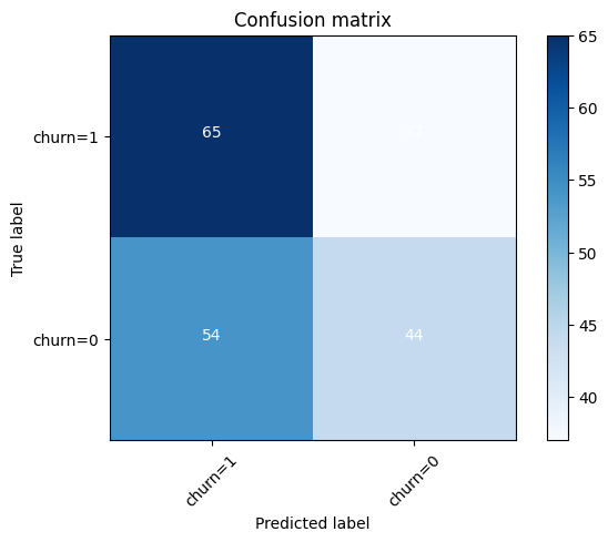
Confusion Matrix : A Confusion Matrix is a fundamental tool used in classification problems to evaluate the performance of a model. It provides a matrix showing the number of correct and incorrect predictions made by the model, categorized by the actual and predicted classes. Where
- True Positive (TP): Correctly predicted positive class (class 1).
- True Negative (TN): Correctly predicted negative class (class 0).
- False Positive (FP): Incorrectly predicted as positive (class 1), but the actual class is negative (class 0). This is also called a Type I error.
- False Negative (FN): Incorrectly predicted as negative (class 0), but the actual class is positive (class 1). This is also called a Type II error.
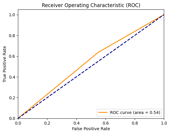
ROC Curve (Receiver Operating Characteristic Curve): The ROC Curve is a graphical representation used to evaluate the performance of a binary classification model across all classification thresholds. It plots two metrics:
- True Positive Rate (TPR) or Recall (Sensitivity)-It is the proportion of actual positive instances (class 1) that were correctly classified as positive by the model.
- False Positive Rate (FPR)-It is the proportion of actual negative instances (class 0) that were incorrectly classified as positive by the model.
AUC: AUC stands for Area Under the Curve and is a performance metric used to evaluate the quality of a binary classification model. Specifically, it refers to the area under the ROC curve (Receiver Operating Characteristic curve), which plots the True Positive Rate (TPR) versus the False Positive Rate (FPR) for different threshold values.
Classification Report: A Classification Report is a summary of various classification metrics, which are useful for evaluating the performance of a classifier on the given dataset.
Task 5: Implementation
Write code to visualize the model’s performance using confusion matrices and ROC curves. Generate classification reports to evaluate precision, recall, and F1-score. Retrain the model with L2 regularization and evaluate the performance.
from sklearn.metrics import classification_report, confusion_matrix, roc_curve, auc
import itertools
import numpy as np

# confusion matrix
def plot_confusion_matrix(cm, classes,
                          normalize=False,
                          title='Confusion matrix',
                          cmap=plt.cm.Blues):
    """
    This function prints and plots the confusion matrix.
    Normalization can be applied by setting `normalize=True`.
    """
    if normalize:
        cm = cm.astype('float') / cm.sum(axis=1)[:, np.newaxis]
        print("Normalized confusion matrix")
    else:
        print('Confusion matrix, without normalization')

    print(cm)

    plt.imshow(cm, interpolation='nearest', cmap=cmap)
    plt.title(title)
    plt.colorbar()
    tick_marks = np.arange(len(classes))
    plt.xticks(tick_marks, classes, rotation=45)
    plt.yticks(tick_marks, classes)

    fmt = '.2f' if normalize else 'd'
    thresh = cm.max() / 2.
    for i, j in itertools.product(range(cm.shape[0]), range(cm.shape[1])):
        plt.text(j, i, format(cm[i, j], fmt),
                 horizontalalignment="center",
                 color="white" if cm[i, j] > thresh else "black")

    plt.tight_layout()
    plt.ylabel('True label')
    plt.xlabel('Predicted label')

test_label = test_outputs > 0.5
cnf_matrix = confusion_matrix(y_test, test_label, labels=[1,0])
np.set_printoptions(precision=2)
plt.figure()
plot_confusion_matrix(cnf_matrix, classes=['churn=1','churn=0'],normalize= False,  title='Confusion matrix')


# Plot ROC curve
fpr, tpr, thresholds = roc_curve(y_test, test_label)
roc_auc = auc(fpr, tpr)

plt.figure()
plt.plot(fpr, tpr, color='darkorange', lw=2, label=f'ROC curve (area = {roc_auc:.2f})')
plt.plot([0, 1], [0, 1], color='navy', lw=2, linestyle='--')
plt.xlim([0.0, 1.0])
plt.ylim([0.0, 1.05])
plt.xlabel('False Positive Rate')
plt.ylabel('True Positive Rate')
plt.title('Receiver Operating Characteristic (ROC)')
plt.legend(loc="lower right")
plt.show()


# Classification report
print (classification_report(y_test, test_label))
Confusion matrix, without normalization
[[65 37]
 [54 44]]
              precision    recall  f1-score   support

         0.0       0.54      0.45      0.49        98
         1.0       0.55      0.64      0.59       102

    accuracy                           0.55       200
   macro avg       0.54      0.54      0.54       200
weighted avg       0.54      0.55      0.54       200
Step 6: Model Saving and Loading
Task 6: Save and load the trained model.
This task demonstrates the techniques to persist a trained model using torch.save and reload it using torch.load. Evaluating the loaded model ensures that it retains its performance, making it practical for deployment in real-world applications.
- Saving the Model:
- Save the model’s learned weights and biases using torch.save().( e.g. , torch.save(model.state_dict(), ‘your_model_name.pth’))
- Saving only the state dictionary (model parameters) is preferred because it’s more flexible and efficient than saving the entire model object.
- Loading the Model:
- Create a new model instance (e.g.,
model = LogisticRegressionModel()) and load the saved parameters. ( e.g. ,model.load_state_dict(torch.load('your_model_name.pth'))).
- Create a new model instance (e.g.,
- Evaluating the Loaded Model:
- After loading, set the model to evaluation mode by calling
model.eval() - After loading the model, evaluate it again on the test dataset to make sure it performs similarly to when it was first trained..Now evaluate it on the test data.
- Use
torch.no_grad()to ensure that no gradients are computed.
- After loading, set the model to evaluation mode by calling
Task 6: Implementation
Write code to save the trained model and reload it. Ensure the loaded model performs consistently by evaluating it on the test dataset.
# Save the model
torch.save(model.state_dict(), 'your_model_name.pth')

# Load the model
model = LogisticRegressionModel(input_dim)
model.load_state_dict(torch.load('your_model_name.pth'))

# Ensure the loaded model is in evaluation mode

model.eval()
with torch.no_grad():
    test_outputs = model(X_test)

# Evaluate the loaded model
test_label = test_outputs > 0.5

print("Test accuracy : ", (test_label == y_test).float().mean())
Step 7: Hyperparameter Tuning
Task 7: Perform hyperparameter tuning to find the best learning rate.
By testing different learning rates, you will identify the optimal rate that provides the best test accuracy. This fine-tuning is crucial for enhancing model performance .
- Define Learning Rates:
- Choose these learning rates to test ,[0.01, 0.05, 0.1]
- Reinitialize the Model for Each Learning Rate:
- For each learning rate, you’ll need to reinitialize the model and optimizer e.g.(
torch.optim.SGD(model.parameters(), lr=lr)). - Each new learning rate requires reinitializing the model since the optimizer and its parameters are linked to the learning rate.
- For each learning rate, you’ll need to reinitialize the model and optimizer e.g.(
- Train the Model for Each Learning Rate:
- Train the model for a fixed number of epochs (e.g., 50 or 100 epochs) for each learning rate, and compute the accuracy on the test set.
- Track the test accuracy for each learning rate and identify which one yields the best performance.
- Evaluate and Compare:
- After training with each learning rate, compare the test accuracy for each configuration.
- Report the learning rate that gives the highest test accuracy
Task 7: Implementation
Perform hyperparameter tuning to find the best learning rate. Retrain the model for each learning rate and evaluate its performance to identify the optimal rate.
learning_rates = [0.01, 0.05, 0.1]
best_accuracy = 0
best_lr = 0

for lr in learning_rates:

    model = LogisticRegressionModel(input_dim)
    criterion = nn.BCELoss()
    optimizer = torch.optim.SGD(model.parameters(), lr=0.01)

    epochs=1000
    for epoch in range(epochs):
        model.train()
        optimizer.zero_grad()
        outputs = model(X_train)
        loss = criterion(outputs, y_train)
        loss.backward()
        optimizer.step()
        if (epoch-1) % 100 == 0:
            print(f'{lr=}, {epoch=}, loss={loss.item()}')

    model.eval()
    with torch.no_grad():
        train_outputs = model(X_train)
        test_outputs = model(X_test)

        train_label = train_outputs > 0.5
        test_label = test_outputs > 0.5
        test_accuracy = (test_label == y_test).float().mean()
        print("Test accuracy : ", test_accuracy)

        if (test_accuracy > best_accuracy):
            best_accuracy = test_accuracy
            best_lr = lr
print(f'{best_lr=}, {best_accuracy=}')
lr=0.01, epoch=1, loss=0.7272074818611145
lr=0.01, epoch=101, loss=0.7126162648200989
lr=0.01, epoch=201, loss=0.7036827206611633
lr=0.01, epoch=301, loss=0.6982945203781128
lr=0.01, epoch=401, loss=0.6950703263282776
lr=0.01, epoch=501, loss=0.6931479573249817
lr=0.01, epoch=601, loss=0.692002534866333
lr=0.01, epoch=701, loss=0.6913199424743652
lr=0.01, epoch=801, loss=0.6909125447273254
lr=0.01, epoch=901, loss=0.6906691193580627
Test accuracy :  tensor(0.5250)
lr=0.05, epoch=1, loss=0.7290753126144409
lr=0.05, epoch=101, loss=0.7147523760795593
lr=0.05, epoch=201, loss=0.7055988311767578
lr=0.05, epoch=301, loss=0.6998367309570312
lr=0.05, epoch=401, loss=0.6962400674819946
lr=0.05, epoch=501, loss=0.6940035820007324
lr=0.05, epoch=601, loss=0.6926141977310181
lr=0.05, epoch=701, loss=0.691750168800354
lr=0.05, epoch=801, loss=0.6912119388580322
lr=0.05, epoch=901, loss=0.6908755302429199
Test accuracy :  tensor(0.5300)
lr=0.1, epoch=1, loss=0.7289024591445923
lr=0.1, epoch=101, loss=0.714150607585907
lr=0.1, epoch=201, loss=0.7048901319503784
lr=0.1, epoch=301, loss=0.6991775631904602
lr=0.1, epoch=401, loss=0.6956901550292969
lr=0.1, epoch=501, loss=0.6935731768608093
lr=0.1, epoch=601, loss=0.6922907829284668
lr=0.1, epoch=701, loss=0.6915143728256226
lr=0.1, epoch=801, loss=0.6910433769226074
lr=0.1, epoch=901, loss=0.690757155418396
Test accuracy :  tensor(0.5400)
best_lr=0.1, best_accuracy=tensor(0.5400)
Step 8: Feature Importance
Task 8: Evaluate feature importance to understand the impact of each feature on the prediction.
The code to evaluate feature importance to understand the impact of each feature on the prediction.
- Extracting Model Weights:
- The weights of the logistic regression model represent the importance of each feature in making predictions. These weights are stored in the model’s linear layer (
model.linear.weight). - You can extract the weights using
model.linear.weight.data.numpy()and flatten the resulting tensor to get a 1D array of feature importances.
- The weights of the logistic regression model represent the importance of each feature in making predictions. These weights are stored in the model’s linear layer (
- Creating a DataFrame:
- Create a pandas DataFrame with two columns: one for the feature names and the other for their corresponding importance values (i.e., the learned weights).
- Ensure the features are aligned with their names in your dataset (e.g.,
X_train.columns).
- Sorting and Plotting Feature Importance:
- Sort the features based on the absolute value of their importance (weights) to identify the most impactful features.
- Use a bar plot (via
matplotlib) to visualize the sorted feature importances, with the feature names on the y-axis and importance values on the x-axis.
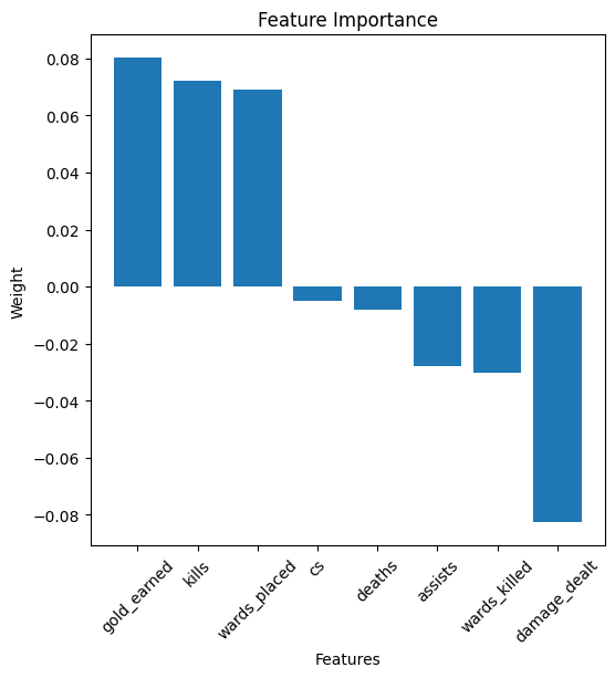
- Interpreting the Results:
- Larger absolute weights indicate more influential features. Positive weights suggest a positive correlation with the outcome (likely to predict the positive class), while negative weights suggest the opposite.
Task 8: Implementation
Evaluate feature importance by extracting the weights of the linear layer and creating a DataFrame to display the importance of each feature. Visualize the feature importance using a bar plot.
import pandas as pd
import matplotlib.pyplot as plt

# Extract the weights of the linear layer
## Write your code here
w = model.linear.weight.data.numpy().flatten()

# Create a DataFrame for feature importance
## Write your code here
df_w = pd.DataFrame({'Feature' : X.columns,'Weight':w})
df_w = df_w.sort_values('Weight', ascending=False)

print(df_w)

# Plot feature importance
plt.figure(figsize=(6, 6))
plt.bar(df_w['Feature'], df_w['Weight'])
plt.xlabel('Features')
plt.ylabel('Weight')
plt.title('Feature Importance')
plt.xticks(rotation=45)
plt.show()
        Feature    Weight
3   gold_earned  0.080194
0         kills  0.072249
5  wards_placed  0.068960
4            cs -0.004865
1        deaths -0.008046
2       assists -0.027868
6  wards_killed -0.030438
7  damage_dealt -0.082819